Cupping correction
This example illustrates how to apply empirical cupping correction using the algorithm of Kachelriess et al. named WaterPrecorrection in RTK. The example uses a Gate simulation using the fixed forced detection actor.
The simulation implements a 120 kV beam, a detector with 512x3 pixels and an energy response curve. Only the primary beam is simulated.
The simulation files, the output projections and the processing script are available here.
#!/usr/bin/env python
import itk
from itk import RTK as rtk
import os
import matplotlib.pyplot as plt
import numpy as np
import scipy.optimize
import glob
# Script parameters
directory = "output/"
spacing = [0.5] * 3
size = [512, 1, 512]
order = 6
reference_attenuation = 0.02
origin = [-(size[0] / 2 + 0.5) * spacing[0], 0.0, -(size[2] / 2 + 0.5) * spacing[2]]
# List of filenames
file_names = list()
for file in os.listdir(directory):
if file.startswith("attenuation") and file.endswith(".mha"):
file_names.append(directory + file)
# Read in full geometry
geometry = rtk.read_geometry("output/geometry.xml")
# Crate template image
ImageType = itk.Image[itk.F, 3]
projections_reader = rtk.ProjectionsReader[ImageType].New(file_names=file_names)
projections = projections_reader.GetOutput()
constant_image_filter = rtk.ConstantImageSource[ImageType].New(
origin=origin, spacing=spacing, size=size
)
constant_image = constant_image_filter.GetOutput()
template = rtk.draw_ellipsoid_image_filter(
constant_image, density=reference_attenuation, axis=[100, 0, 100]
)
itk.imwrite(template, "template.mha")
template = itk.array_from_image(template).flatten()
# Create weights (where the template should match)
weights = rtk.draw_ellipsoid_image_filter(
constant_image, density=1.0, axis=[125, 0, 125]
)
weights = rtk.draw_ellipsoid_image_filter(weights, density=-1.0, axis=[102, 0, 102])
weights = rtk.draw_ellipsoid_image_filter(weights, density=1.0, axis=[98, 0, 98])
itk.imwrite(weights, "weights.mha")
weights = itk.array_from_image(weights).flatten()
# Create reconstructed images
wpcoeffs = np.zeros(order + 1)
fdks = [None] * (order + 1)
for o in range(0, order + 1):
wpcoeffs[o - 1] = 0.0
wpcoeffs[o] = 1.0
water_precorrection = rtk.water_precorrection_image_filter(
projections, coefficients=wpcoeffs, in_place=False
)
fdk = rtk.fdk_cone_beam_reconstruction_filter(
constant_image, water_precorrection, geometry=geometry
)
itk.imwrite(fdk, f"fdk{o}.mha")
fdks[o] = itk.array_from_image(fdk).flatten()
# Create and solve the linear system of equation B.c= a to find the coeffs c
a = np.zeros(order + 1)
B = np.zeros((order + 1, order + 1))
for i in range(0, order + 1):
a[i] = np.sum(weights * fdks[i] * template)
for j in np.arange(i, order + 1):
B[i, j] = np.sum(weights * fdks[i] * fdks[j])
B[j, i] = B[i, j]
c = np.linalg.solve(B, a)
water_precorrection = rtk.water_precorrection_image_filter(projections, coefficients=c)
fdk = rtk.fdk_cone_beam_reconstruction_filter(
constant_image, water_precorrection, geometry=geometry
)
itk.imwrite(fdk, "fdk.mha")
fdk = itk.imread("fdk.mha")
fdk1 = itk.imread("fdk1.mha")
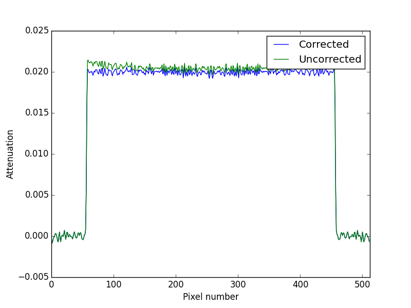
plt.plot(itk.array_from_image(fdk)[:, 0, 256], label="Corrected")
plt.plot(itk.array_from_image(fdk1)[:, 0, 256], label="Uncorrected")
plt.legend()
plt.xlabel("Pixel number")
plt.ylabel("Attenuation")
plt.xlim(0, 512)
plt.savefig("profile.png")
The resulting central profiles are